GraphSage

Graphs have been used across many fields due to their ability to represent relationships between entities with applications including social networks, search engines, and protein-protein interaction networks. However, one growing limitation of these graphs are the amount of computational resources they require with some large-scale graphs having millions of nodes each with their own set of features and their set of edges.
This has led to the creation of graph embedding methods, more specifically the deep embedding methods. These embedding methods aim to create a high-quality representation of the nodes and their edges. Rather than just incorporating the graph structural information into an embedding, these methods also include node and edges features and other hierarchical information. This results in a complicated model which are able to learn very rich representations of nodes.
Deep embedding methods use neural networks called graph neural networks (GNNs) to create these deep embeddings. GNNs consists of many layers, with each layer consisting of a message passing (neighbourhood aggregation) system and an update function. The message passing aggregates the information from its neighbours while the update function use these aggregations to update the node's current representation within the layer.
There are many different GNNs with many specialised for different tasks. Some incorporate temporal dynamics, others incorporate attention mechanisms, some are built for different scales, etcetera. From these GNNs, today we will be looking at GraphSage by Hamilton et al..
Inductive vs Transductive Methods
From the GNN node embeddings methods, they can often be split into 2 categories: transductive and inductive methods. Transductive methods create embeddings from the nodes it has seen during training but they are unable to generalise to nodes they have not seen. To create embeddings for new nodes, the GNN would have to be retrained on these new nodes. On the other hand, the inductive methods can generalise to nodes they have never encountered before. As a result the inductive methods are computationally efficient compared to transductive methods and perform better with dynamic graphs.
GraphSage (SAmple and aggreGatE) was one of the first successful inductive node embedding algorithms. It was inspired by a variant of the Graph Convolution Network (GCN), another inductive GNN method.
Rather than training a distinct embedding vector for each node, a set of aggregate functions are trained to incorporate the structural and node features.
GraphSage introduced 2 methods: the embedding generation method (called the forward propagation algorithm) and model parameter training method.
Forward Propagation Algorithm
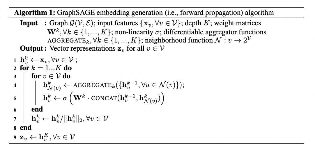
Given a Graph $\mathcal{G}(V, \mathcal{E})$ where $V$ corresponds to the domain of nodes and $\mathcal{E}$ corresponds to the domain of edges. The embedding generation method follows:

The intuition behind this approach is as each iteration continues, the nodes continue to aggregate information from their local neighbours and stores the information for node $v$ in layer $k$ of the algorithm in an embedding vector $h_{v}^{k}$. As this process continues, more information about the whole graph is aggregated.
Model Parameter Training
To allow this method to work in the mini batch setting, given a mini batch of size $m$ and it's batch of nodes $\{ v_{1}, ..., v_{m} \}$, rather than iterating over all nodes in the graph, only the nodes needed up to a depth K are used.
To train the parameters of the model, Hamilton et al. used a loss function inspired by vector calculus. Given a node $u$ and it's final node embedding of $z_{u}$, the loss function can be defined as:
$$J_{\mathcal{G}}(z_{u}) = -\log(\sigma(z_{u}^{T} z_{v})) - Q\cdot \mathbb{E}_{v _{n} \sim P_{n}(v)} \log (\sigma(-z_{u}^{T} z_{v_{n}})).$$
where $v$ is a node that co-occurs near $u$ on a fixed-length random walk, $\sigma$ is the sigmoid activation function, $P_{n}$ is the negative sampling distribution, and $Q$ defines the number of negative samples. This form of loss encourages nodes which close to $u$ to have similar embeddings, while nodes far away to be distinguishable. To see this, we'll write the loss function using the sigmoid activation function.
$$J_{\mathcal{G}}(z_{u}) = \log(1 + e^{-z_{u}^{T} z_{v}})) + Q\cdot \mathbb{E}_{v _{n} \sim P_{n}(v)} \log (1 + e^{z_{u}^{T} z_{v_{n}}})).$$
The term on the left: $1 + e^{-z_{u}^{T} z_{v}}$ achieves a maximum of 2 when the vectors are orthogonal and when the vector embeddings are parallel, the minimum of $1 + e^{-1}$ is achieved.
Similarly, the term $1 + e^{z_{u}^{T} z_{v_{n}}}$ is minimised with the value of 1 when the vectors are orthogonal and maximised when the vectors are parallel.
The key difference to previous method which have implemented this form of loss is that here, we restrict the embeddings $z_{u}$ to be the embeddings generated from the features contained within a node's local neighbourhood, unlike generating a unique embedding for each node.
GraphSage Aggregation Functions
Similar to other GNN algorithms, GraphSage's aggregator function had to be symmetric, trainable, and have the ability to provide a rich representational capacity. So GraphSage experimented with 3 different aggregator functions: the mean aggregator, LSTM aggregator, and the pooling aggregator.
Mean Aggregator
Given embedding vectors$\{ h_{u}^{k-1}, \forall u \in \mathcal{N}(v) \}$, the mean aggregator for the embedding for node v and layer k is written as:
$$ h_{v}^{k} \leftarrow \sigma (W \cdot \text{MEAN}( \{h_{v}^{k-1}\} \cup \{ \{h_{u}^{k-1}, \forall u \in \mathcal{N}(v) \})).$$
This method is often referenced as the mean based aggregator convolutional since it is rough linear approximation of the local spectral convolution (see the appendix).
LSTM Aggregator
Another experimented aggregator function was the LSTM (see the appendix) aggregator. Here LSTMs have the advantage of having more expressive capabilities but suffers from its main limitation of being inherently non-symmetric due to their sequential processing. To help the LSTM overcome this limitation, a random permutation of the node's neighbours are inputted to LSTM.
Pooling Aggregator
The final of the 3 approaches is the pooling approach where a neighbouring embeddings are fed independently through a neural network:
$$\text{AGGREGATE}_{k}^{\text{pool}} = \max(\{ \sigma(W _{\text{pool}} h_{u_{i}}^{k} + b), \forall u_{i} \in \mathcal{N}(v) \}),$$
where the max is the element-wise max operator and sigma is a non-linear activation function.
Results
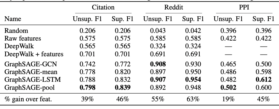
The authors Hamilton et al. tested the performance on 3 benchmark datasets, classification of academic papers, classifying Reddit posts, and classifying protein functions. For each dataset, the 3 variants of GraphSage were trained along with using a variant inspired by the GCN. Each of these methods were compared to DeepWalk by Perozzi et al. (see the appendix).
Two further variants of the GraphSage model were tested: the unsupervised model which was trained on the loss function defined above and the supervised model which was trained on the cross-entropy loss function. For further insights into the experimental details, visit Hamilton et al.'s paper.

From the results, each of the tested aggregators exceeded the performance of the previous state of the art methods with the GraphSage-LSTM and GraphSage-pool achieving the highest results.
Conclusion
This article delved into GraphSage, an inductive node embedding method with applications in large scale graph.
Appendix
Spectral Convolution: In spectral graph convolution, an eigen decomposition of the Laplacian matrix is performed, which gives us the information related to the underlying structure of the graph. This operation is performed on the Fourier space and finds the smallest eigenvalues as these explain the graph structure better in Spectral Convolution. ChebNet is an example of a method which has applied the idea spectral convolutions with a focus on local spectral convolutions.
Local Spectral Convolution: The difference between spectral convolutions and local spectral convolutions is that the local methods focus more on the informations from a node's immediate neighbourhood rather than the entire graph. As a result these methods are more computationally efficient and often provide more practical relevance. The Graph Convolution Network (GCN) used a first-order approximation of the spectral convolution which lead to localised operations. Here the full-spectral convolution can be written as:
$$h_{v} = \sum_{u\in \mathcal{N}(i)} \frac{1}{\sqrt{d_{u}d_{v}}} h_{j},$$
where $d_{v}$ and $d_{u}$ correspond to the degrees of nodes v and u.
Spatial Convolution: These methods work on local neighbourhoods of nodes to understand their properties based on the k neighbours. Unlike spatial convolutions, these methods are much simpler to implement. GraphSage is an example of Spatial Convolution.
Negative Sampling: Negative sampling is a technique in machine learning which is designed to enhance the efficiency of the models by selecting a small subset of negative samples from a pool of negative samples. This form of loss function is defined the maximise the similarity between the positive pairs and minimise the similarity between the negative pairs. As a result, this form of model should be able to distinguish between positive and negative samples, in our case, between nodes close and far apart.
DeepWalk: DeepWalk is a shallow node embeddings method which uses a random walk to capture the nodes structure. These random walks sequences are then applied to the Skip-Gram model to predict nearby nodes. Using the Skip-Gram model, dense vector embeddings for the nodes are generated where nodes that co-occur have a similar embedding.
LSTM: An LSTM is a type of recurrent neural network (RNN) that is designed to better capture and retain information while avoiding the vanishing gradient problem. There LSTM is composed of 3 gates, the forget gate, input gate, and output gate, with each gate controlling the amount of information to be stored or forgotten during each step.
References
Hamilton, W., Ying, R. and Leskovec, J. (n.d.). Inductive Representation Learning on Large Graphs. [online] Available at: https://arxiv.org/pdf/1706.02216 [Accessed 11 Sep. 2024].
Perozzi, B., Al-Rfou, R. and Skiena, S. (n.d.). DeepWalk: Online Learning of Social Representations. [online] doi:https://doi.org/10.1145/2623330.
Hochreiter, S. and Schmidhuber, J. (1997). Long Short-Term Memory. Neural Computation, 9(8), pp.1735–1780. doi:https://doi.org/10.1162/neco.1997.9.8.1735.
in (2019). What is the difference between graph convolution in the spatial vs spectral domain? [online] Artificial Intelligence Stack Exchange. Available at: https://ai.stackexchange.com/questions/14003/what-is-the-difference-between-graph-convolution-in-the-spatial-vs-spectral-doma [Accessed 11 Sep. 2024].